=========================================================================================
Trackml Challenge
This is my 16th place solution for the TrackML Particle Tracking Challenge on Kaggle.
The Challenge
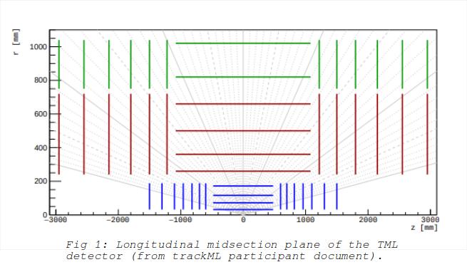
The challenge is to identify the tracks of particles that are created from colliding protons. The collisions take place at the origin (xyz coordinates) inside a cylindrical structure that is made up of many detectors. These detectors provide the position of a particle as it moves through them. Each detected position of a particle is referred to as a ‘hit’. The detectors are organized as ‘volumes’, which contain ‘layers’, which contain ‘modules’, each module is composed of many detector cells. The shape of a volume can be cylindrical or disc shaped seen in fig 1. The particles move through a relatively constant magnetic field so the expected paths are helical depending on the amount of charge on the particle.
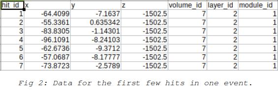
The data which is provided is divided into many csv files, each of which contains the hit data for one collision event. The task is to assign a track to each hit where each track represents one particle. This is done separately for each event. There are also supplementary files for each event that provide the ground-truth, particle and cell information for each event. The hit data consists mainly of the x,y,z coordinates for the detected hit as well as the volume, layer and module information for the detector involved. An example of this is shown in fig 2.
The solution approach The approaches that most interested me were neural nets, hough transforms, and clustering. I didn’t think that it would be possible to get a good score using a strictly neural net approach such as a cnn. A cnn is good at finding useful features in the data as it is being trained. But in this case we actually have exact information to create features from the data, namely the helical path that a particle takes as it moves. A neural net for clustering the hit data after features have been created might be more promising, but I did not spend time on this approach. I experimented with a hough transform approach but found that the large number of calculations just took too much time to make it practical.
The approach that I settled on was clustering using dbscan. My script used the helix unrolling approach provided in Grzegorz Sionkowski’s script. Since particles move in a helix along the z axis, they are rotating around a center in the xy plane. This means that at any position on the helix a particle has rotated around the center of a circle by an amount that is proportional to the distance traveled along the z axis. So subtracting this angle of rotation should bring the particle back to the starting angle at the origin. The clustering is then done on features calculated after this unrolling. The features discussed on the forums included the starting angle and the ratio of z to the xy distance or the xyz distance. The ratio features don’t take into account the curvature of the track so they will not work that well for tracks that have a more pronounced curvature.
In order to use better features I came up with features that are based on the helical nature of the tracks. In the xy plane a particle travels in a circle as it moves along the helix. This is illustrated in fig 3.
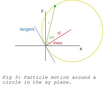
Since the unrolling operation moves the particle position back to the starting point at the origin the angle made with respect to the origin is the same as the angle made by the tangent to the circle at the origin. This allows us to obtain the angle made by the radius of the circle with respect to the origin, theta is offset from the tangent by 90 degrees. Since r and phi can be computed from the x and y coordinates of the hit point we can then calculate the value of r0 (or it’s inverse). The following equations are used in calculating features for the dbscan clustering algorithm.
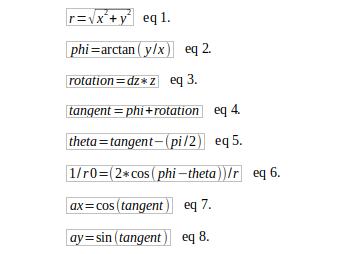
The three features selected for dbscan are ax,ay and 1/r0. The ax and ay are chosen instead of the tangent angle to avoid issues with two angles of different values even though they are very similar, such as 0 and 359 degrees.
The clustering is done over many iterations within nested loops that vary the different parameters used in capturing tracks. At each iteration all points that have been assigned tracks are removed from the pool of available points. The idea here is that these points will no longer be available to be incorrectly assigned to some other track by later iterations. The order of the nested loops is as follows, outer loops first: Iterate over decreasing values of the minimum cluster size that is accepted as a valid track. Iterate over increasing values of epsilon used in dbscan. Iterate over each z-offset value, starting with 0, then gradually increasing the offset, alternating between positive and negative values. Iterate over increasing values of rotation rate for calculating the tangent.
To increase the size of tracks discovered by dbscan some track extension was also implemented. This was inspired by Heng CherKeng’s track extension script, where the track is extended at the two endpoints (minimum and maximum z). Instead of doing this after all clusters have been found, I opted to extend each track immediately after it has been assigned by dbscan. The extension is done by finding points that are close feature-wise to the minimum and maximum point.
Credits:
https://www.kaggle.com/sionek/mod-dbscan-x-100-parallel
https://www.kaggle.com/c/trackml-particle-identification/discussion/58194
The code is available at https://github.com/robert604/Trackml
Text Normalization Challenge
This is my 19th place solution for the english text normalization challenge on Kaggle. The task is to convert written text into a spoken form. The data consists of sentences that have been broken down into tokens where each token has to be normalized. An example of a sentence from the training data is shown below.
| sentence_id | token_id | class | before | after |
|---|---|---|---|---|
| 997 | 0 | PLAIN | Library | Library |
| 997 | 1 | PLAIN | of | of |
| 997 | 2 | PLAIN | Congress | Congress |
| 997 | 3 | PLAIN | number | number |
| 997 | 4 | TELEPHONE | 77-96925 | seven seven sil nine six nine two five |
| 997 | 5 | PUNCT | . | . |
The “before” column contains each text token before conversion and the “after” column is the normalized version.
Looking at the objective
The required task for this competition is to correctly specify the spoken form of the tokens which make up sentences. In most sentences the majority of the tokens remain unchanged.
A straight forward translation of a single input to a single output would not be practical because of the very different transformations required for different cases. The types of transformations required can be broken down into two main categories, replacements and transformations. In the case of replacements we are replacing the input token with fixed strings. There are three possibilities.
Same replace: The output text is exactly the same as the input.
Single replace: The output text is different from the input, but it is always the same for the same input. For example ‘privatise’ is replaced by ‘privatize’.
Multi replace: There are tokens which have more than one possible string as the output, so the correct one would have to be chosen based on the context in the sentence. For example ‘st’ can have either ‘saint’ or ‘street’ as a replacement.
In order to do these replacements we need to have the replacement strings available in advance, so this is only possible for tokens that occur in the training set. For ‘Single’ and ‘Multi’ replace it is straight forwards to create a dictionary of tokens and their replacements using the data available at training time. For ‘Same’ replacements though, there will also be tokens in the test set that are not to be found in training data. These tokens would have to be identified by a classifier as being candidates for ‘Same’ replacement.
Aside from tokens that can be replaced with text constants, there are also tokens for which the output is not a replacement but is generated from the input token. In cases like these an input token from the test set that does not occur in the training set needs to undergo the same transformation, since it’s replacement is not available. Obviously all types of transformations have to be known in advance. An example of a transformation for a number is ‘20’ which is transformed to ‘twenty’. Transformations are also applied to words and other types of text, such as dates.
The majority of the transformations or replacements can be identified and done without any kind of machine learning, but some type of classifier is needed for the remaining few where the type of transformation needed is not so obvious. For example most purely alphabetic tokens end up unchanged but there are some that must be transformed in some way, such as being spelled as letters. These exceptions are the ones that need to be identified based on the context surrounding the token.
The overall approach
The approach which seems best for this problem is to first determine what type of replacement or transformation is needed and then apply it. We know that if the correct replacement or transformation is applied the output will always be correct. So the difficult part then is to classify a token and determine the appropriate operation to get the output. The training set does include a ‘class’ column which categorizes the token into classes for transformation. This information is not available for the test set.
The different classes are:
‘PLAIN’, ‘PUNCT’, ‘DATE’, ‘LETTERS’, ‘CARDINAL’, ‘VERBATIM’, ‘DECIMAL’, ‘MEASURE’, ‘MONEY’, ‘ORDINAL’, ‘TIME’, ‘ELECTRONIC’, ‘DIGIT’, ‘FRACTION’, ‘TELEPHONE’, ‘ADDRESS’
Looking at some of the classes in the data I could see that simply using these categories for determining transformations was not going to be adequate. The reason being that for many of the classes there can be more than one possible transformation to be applied. For example the token “XXIII” in the ORDINAL class can be transformed into ‘the twenty third’ as well as ‘twenty third’. Also this same token exists in the CARDINAL class and is transformed into “twenty three”. So there are a total of three possible transformations.
Reclassing
For this token then, a better approach would be to have three classes, one for each type of transformation. With this in mind I categorized the dataset into about 40 classes where each class represents one type of transformation. Aside from the one class to one transformation benefit, this method also eliminates the need to include some of the new classes in the classifier. This is because these classes can be determined simply by using regex methods. For example, if we look at the date tokens, the input token ‘19 July 1946’ which transforms to ‘the nineteenth of july nineteen forty six’ is guaranteed to not be mistaken for any other class. So it can be detected and transformed without ever being considered by the classifier, making it’s job easier.
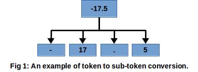
Sub-tokens
Since all input tokens are categorical, one issue that arises is that it is hard for the classifier to distinguish between tokens of different types. It is hard to distinguish between alphabetic tokens, numeric tokens, punctuation tokens, or tokens that are a mixture of different types. Another issue is that of generalization. If we have the token ‘12345’ in the train set the classifier could learn that it is a number and should be categorized as one of the number classes. But this does not help it classify the token ‘54321’ if it only shows up in the test set. To make it easier for the classifier to recognize token types each token is split up into sub-tokens. This is done by splitting the token text into words, numbers and punctuation characters etc. A maximum of 10 sub-tokens are produced for each token. Fig 1 shows an example of this.
The classifier
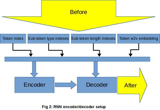
For the classification portion of this task I decided to go with an LSTM based neural net. The net uses an encoder and decoder approach with attention. I used Pytorch because of it’s flexibility which made it easier I think to implement the attention code and some other features. The inputs to the neural net are:
- The token index.
- The sub-token type index.
- The sub-token length index.
- The word2vec embedding for the token.
All categorical indexes are fed into embeddings layers in the encoder and decoder. This setup can be seen in fig 2.
Limiting output types
If you take a look at tokens in the dataset you might realize that for most tokens we can only classify them as one or more classes which are a subset of all the classes. Meaning that we can exclude many of the classes for consideration. For example the number ‘12345’ should only be classified as some kind of number class and should not ever be classified as an alphabetic type class. Limiting the outputs of the neural net so that only valid classes are allowed means an increase in classification accuracy. I implemented this type of class limiting by adding a large positive constant to the raw probabilities of the valid classes (before softmax) which had been output by the neural net. This ensures that the class with the highest probability will be one of the valid classes.
Ensembling sort of…
The majority class in this dataset is the one for ‘same replacement’. In order to do some kind of ensembling I trained two models. The first model, was trained without any compensation for the class imbalance so it was good at classifying the majority class at the expense of the less frequently occuring classes. The second model, was trained with the same data but only a percentage of the tokens for the most frequent class (selected at random) have their error used in updating the weights of the network. This focuses the network on learning to classify the less frequent classes at the expense of the more frequent ones. When generating the final output the predictions from the first model are used for ‘same replacement’ , while predictions for all other classes are taken from the second model.
Training and validation
For testing locally the train set was split up with 20% of the data used for validation. The optimizers used for the encoder and decoder were Adam optimizers, and the loss function was cross entropy loss. A batch size of 64 was chosen and each model was trained for 10 epochs. I didn’t get a chance to do any fine-tuning which I think would have improved my score. When training for the actual test set the entire train set was used for training the neural net. It took about 6 hours to train two models on a GTX1060 gpu.
In addition to the data made available for the competition I also made use of the publicly available data on github for creating the replacement dictionaries. This was an improvement over making the dictionaries using only the train set.
The code is available at https://github.com/robert604/text_normalization